


How fast can one machine search a quarter of a billion vectors that don't fit in its RAM? We went and measured it: SereneDB was faster than Qdrant in 32 of the 33 rows both engines answer, by 1.3× to 14×.
We took all of Cohere's multilingual Wikipedia: 246,838,423 paragraphs, each embedded into 1024 floats. That's a terabyte of vectors on a machine with 185 GB of RAM. Both engines got the fastest layout that fits at this size. It keeps a compact copy in RAM: an HNSW graph, which links each vector to its nearest neighbours for a query to walk, built over 2-bit codes of the vectors. A query walks the graph on the codes in memory, then reranks its best candidates with the full vectors. Only that last step reads from disk. We loaded the data into SereneDB 26.11.1 and into Qdrant 1.20.0, one of the fastest open-source vector databases, with the same index settings in both. Then we sent both the same queries, without a filter or with one of ten kinds of filters, asking for up to 1000 neighbours at recall from 0.90 to 0.99. To know the right answers we computed the exact top 1000 of every query by brute force over all 247 million vectors, once for every filter. Every query was timed exactly once, because a query run twice is answered the second time from the page cache. After that we did it all again on the first 10 million paragraphs, which do fit in RAM, to see how the engines do when the disk isn't involved.
Here's why we care. If you do vector search today, you probably run a dedicated vector database next to your main one, copy the embeddings over along with every field your filters need and then keep the two in sync. We doubt you need that. In SereneDB an embedding is just a column and HNSW is one column of the same index that serves full-text search and filters. The usual argument for a second system is speed, so this benchmark is also a test of that argument.
TL;DR
On 247 million vectors SereneDB is faster in 32 of the 33 rows both engines answer, by 1.3× to 14×. The 33rd is a tie on exact search, where both engines wait on the disk. Five more rows only SereneDB gets to the target recall. Three of them are on the 0.1% filter, where Qdrant finds almost none of the true neighbours at any beam. In the other two Qdrant never reaches recall 0.99. The lead grows with k, because Qdrant rereads several times more vector data from disk per query. On 10 million vectors in RAM, SereneDB is faster in all 20 rows both reach, by 1.5× to 9.2×. It's also the only one to reach recall 0.95 in 11 more.
At 10 million vectors Qdrant needed no special care. At 247 million it needed four non-default settings and 10.6 hours to load, against 5.7 for SereneDB. There a filtered query can stall for up to two minutes when that field's index has left memory.
- Summary
- 247M vectors
- 10M vectors
| 247M, reranked from disk | SereneDB 26.11.1 | Qdrant 1.20.0 |
|---|---|---|
| unfiltered top-10 at recall 0.95 | 521 QPS | 235 QPS |
| load (ingest and index) | 5.7 h | 10.6 h |
| on disk | 1.12 TB | 1.36 TB |
| cold start: accepts queries | 5 s | 277 s |
| cold start: first vector query | 213 s | 277 s |
| filtered query when the field's index is not in memory | 0.02–1.7 s | 98–126 s |
| 10M, everything in RAM | SereneDB 26.11.1 | Qdrant 1.20.0 |
|---|---|---|
| unfiltered top-10 at recall 0.95 | 8,177 QPS | 3,477 QPS |
| load (ingest and index) | 776 s | 778 s |
| cold start: accepts queries | 3 s | 25 s |
| cold start: first vector query | 29 s | 25 s |
The full results are at playground.serenedb.com/vectorbench and every measured point of every curve is in the VectorBench repository.
What VectorBench measures
VectorBench is our open benchmark for vector search in databases, built the way ClickBench is built for analytics: every participant is a directory with its own scripts, settings and queries. Anyone can add one.
The corpus
All of Cohere's wikipedia-2023-11-embed-multilingual-v3: 246,838,423 paragraphs in 323 languages, 1024 dimensions, compared by cosine similarity. That is 1 TB of float vectors. They are unit length, so cosine equals the inner product and both engines are configured for inner product. The 10,000 queries are paragraphs held out from seven languages (English, German, French, Spanish, Russian, Japanese and Chinese). The ground truth is the exact top 1000 for every query and every filter, computed by brute force. The 10M dataset is the first 10 million rows of the same stream, with the same queries and filters and its own ground truth.
The filters
| Filter | Keeps | What it tests |
|---|---|---|
| none | 100% | the graph alone |
cat10 = v | 10% | a common category |
cat100 = v | 1% | a rare category |
cat1000 = v | 0.1% | a very rare one |
num range | 10%, 1% | a range filter |
cat10 = v AND num range | 1% | a conjunction |
| the query's own cluster | ~2% | a filter that agrees with the vector |
| a far cluster | ~0.01% | a filter that fights it |
| the query's language | 1–17% | a real attribute that agrees |
| another language | 1–17% | a real attribute that does not |
Each filter is asked at k = 10, 100 and 1000. Each table row asks for the throughput at recall 0.90, 0.95 or 0.99. That gives 39 rows. One of them, exact search without a filter, is not run: one query reads 1 TB.
How a cell is read
An approximate index trades recall for speed through its search knobs. Each engine declares a ladder of knob values per query group and every point of the ladder is measured. The table reads each engine's own best curve (its Pareto frontier) at the recall the row asks for. Nobody has to agree on knob values: each engine is read at its best.
How we set it up
The machine
One AWS c7i.24xlarge: 96 vCPUs (Xeon Platinum 8488C), 185 GB of RAM and an EBS volume that gives about 560 MB/s and 10,000 IOPS. The 1 TB of float vectors can't be cached on it, so the rerank, which rescores a query's final candidates at full precision, reads them from the volume.
The same index for both
Both engines build HNSW with m = 16 and ef_construction = 256, in 8 segments, over 2-bit TurboQuant codes, which compress each vector to 2 bits per dimension. The graphs and codes stay in RAM, about 100 GB. The float vectors stay on disk. A query walks the graph on codes and then rereads some candidates at full precision from disk to rank them.
This is the layout that gives the best recall per query when the full vectors do not fit in RAM but a graph and compact codes do: the walk never waits for the disk and only the final candidates are read. On a machine with less memory, where even the graph and codes do not fit, the choice changes to fully on-disk indexes, IVF-style partitions or DiskANN-style graphs. That is a different workload with different opponents. We plan to add it to VectorBench as a separate tier.
SereneDB
The rows go into a search table. One inverted index covers the filter columns and the embedding, whose HNSW is one column of that index:
CREATE TABLE items (
  id BIGINT, cat10 SMALLINT, cat100 SMALLINT, cat1000 SMALLINT, num INTEGER,
  ts TIMESTAMP, cluster SMALLINT, lang TEXT, title TEXT, emb FLOAT[1024]
) WITH (storage = 'search');

CREATE INDEX items_vec ON items USING inverted(
  id, cat10, cat100, cat1000, num, cluster, lang,
  emb hnsw (metric = 'ip', quant = 'tq', nb_bits = 2, compression = false, m = 16, ef_construction = 256)
);
compression = false keeps the float vectors uncompressed, like Qdrant's. A query is a prepared SQL statement. The two search knobs are set per session; the filter value, the query vector and k are bound per query:
SET sdb_hnsw_ef_search = 192;
SET sdb_ann_rescore_width = 1;
SELECT id FROM items WHERE cat100 = $1 ORDER BY emb <#> $2 LIMIT $3;
sdb_hnsw_ef_search is the beam. sdb_ann_rescore_width decides what is reread: a candidate is read at full precision only while its code score, widened by width times that code's estimated error, could still beat the k-th exact score found so far. For a filter, the planner decides per segment from the index's own counts whether to walk the graph with the filter or to score the matching rows directly.
Qdrant
One collection with the vectors on disk, the graph in RAM and TurboQuant codes kept in RAM, plus a payload index for every field a filter uses:
client.create_collection(
    "items",
    vectors_config=VectorParams(size=1024, distance=Distance.DOT, on_disk=True),
    hnsw_config=HnswConfigDiff(m=16, ef_construct=256, full_scan_threshold=10000, on_disk=False, payload_m=0),
    optimizers_config=OptimizersConfigDiff(default_segment_number=8, max_segment_size=140_000_000),
    quantization_config=TurboQuantization(turbo=TurboQuantQuantizationConfig(always_ram=True, bits=TurboQuantBitSize.BITS2)),
)
for field in ("cat10", "cat100", "cat1000", "num", "cluster", "lang"):
    client.create_payload_index("items", field, ...)
A query sets the beam (hnsw_ef), turns ACORN on for filtered searches (when the filter rejects a node's direct neighbours, the walk also tries their neighbours) and rescores oversampling × k candidates at full precision:
{"filter": {"must": [{"key": "cat100", "match": {"value": 42}}]},
 "params": {"hnsw_ef": 192, "acorn": true, "quantization": {"rescore": true, "oversampling": 1.0}}}
The payload indexes stay on disk, memory-mapped and read on demand. Everything else is Qdrant's default, except the first four settings below, which this size needed:
payload_m = 0. By default Qdrant adds extra graph links for every value of every indexed field. With six indexed fields on 247 million points those graphs would not fit in memory, if they finished building at all. Withpayload_m = 0, Qdrant, like SereneDB, searches one graph per segment and uses a secondary index for the filter. The 10M run uses it too, so both sizes compare the same design.max_segment_sizeraised, so the collection stays in 8 segments like SereneDB's. We first tried the default: it cut the collection into more than 300 segments and, as expected, gave a worse curve, lower throughput at the same recall, because every query searches every segment and each segment rereads its own candidates.mmap_advicesequential during indexing. With the default random advice the build reads its vectors back one 4 KB page at a time, and the index phase would have taken about a week instead of 6.9 hours. Queries run with the default.- 4 optimization threads during indexing, because with the default the index phase runs out of memory.
async_scorer, Qdrant's io_uring rescorer, stays off, as it is by default: Docker's default seccomp profile blocks io_uring, so most deployments can't use it.
Qdrant at 247 million points
At 10 million points Qdrant was easy: with its defaults it built the index in 7 minutes and nothing above but payload_m was needed. At 247 million it was a different system to run:
- Building needed two workarounds and still filled the machine. With the defaults the build would have taken about a week, reading its vectors one 4 KB page at a time, and it ran out of memory. Even with 4 threads its memory reached 159 GB and left 23 GB free, so we added swap to let the build finish.
- Loading took 10.6 hours: 3.7 to upload the points and 6.9 to build the graphs, against 5.7 hours for SereneDB.
- Filters need opting in. ACORN, Qdrant's filtered walk, is off unless every filtered query turns it on.
- Oversampling doesn't buy recall. Asking Qdrant to rerank twice as many candidates halves its throughput and leaves recall where it was: top-10 at
hnsw_ef512 reaches recall 0.985 at 222 QPS with oversampling 1 and 0.983 at 97 QPS with 2. We explain why below. - Restarts and filters wait on the disk. After a restart Qdrant answers nothing for 277 s. Its payload indexes take 50 GB and a filtered query whose index has left memory stalls for up to two minutes (see below).
Every query is timed once
The vectors do not fit in RAM, so a query that runs twice is answered the second time from the page cache. The measurement follows three rules:
- Each point runs its own queries. The 10,000 queries are shuffled once with a fixed seed. Each point of a group takes the next slice: up to 1,000 queries at k = 10, 500 at k = 100 and 200 at k = 1000, fewer when a group has so many points that the slices would run out. No query runs twice within a group and both engines get the same slices.
- The cache is emptied before every group. All groups ask about the same 10,000 query vectors, so before each group the page cache is dropped and the data files each engine memory-maps are paged out of its own mappings. Graphs and codes stay in RAM.
- Every query of a point runs. There is no warmup and no time limit that cuts a point short. A point that would take more than 15 minutes is left out and listed, not quoted.
The top-10 ladders start at a beam of 16, so each curve covers recall from about 0.8 up. Each engine's graph on the results page also shows the points of the same build answered from the codes alone, without reranking: drawn, never read into the table.
32 clients send queries concurrently. The engines are measured one at a time. The first query of each group runs before the clock starts and is recorded on its own, because Qdrant can stall on it for up to two minutes when that field's payload index is not in memory.
247M: load, size and startup
SereneDB ingests the 247 million rows in 2.5 hours and then merges them into 8 segments in 3.2 hours. Qdrant uploads the points in 3.7 hours and then builds the graphs in 6.9 hours.
The engines also differ in what works between the two phases. SereneDB builds each segment's graph when it writes the segment, so the index answers vector queries from the first rows on. Its rerank works on the candidates of all segments together, so many small segments cost speed rather than recall. Qdrant, loaded with indexing off as its docs advise for bulk uploads, has no graph until the index phase. Until then a query scans every point. Right after the ingest, before the second phase began, we sent each engine top-10 queries from one client. SereneDB answered at recall 0.998, 54 ms per query at the median, once a first query of 208 s had loaded its graphs. Qdrant took 1.4 s per query at the median and up to 114 s.
On disk the two are close: 1.12 TB against 1.36 TB, most of it the 1 TB of float vectors in both.
Startup, from starting a stopped engine with the page cache dropped, happens in different places in the two engines:
SereneDB comes up in seconds and answers everything that does not need a graph right away; the first vector query loads the graphs and codes of all 8 segments, about 100 GB. Qdrant loads the collection eagerly and answers nothing, not even a health check, until it is done.
Filters that wait on the disk
Qdrant keeps its payload indexes memory-mapped and reads them on demand. At this size they are big: 7.6 to 10.8 GB per field, 50 GB for the six. Qdrant maps them with its default random advice, without read-ahead, so an index that is not in memory comes back one 4 KB page at a time. A filtered query waits for that, 98 to 126 s in our runs. It is not a one-time cost per field. It comes back whenever other reads push the index out of memory. Here the rerank alone reads tens of gigabytes per group: the cat10 AND num group waited 126 s although both fields had been used hours before.
SereneDB's filters read only the postings of the value a query asks for. Our eviction drops its index files before every group, so every group starts cold. Its first filtered query still took 0.02 to 1.7 s.
247M: results
Every bar is read off the engine's frontier at the row's recall, in queries per second, and each label ends with SereneDB's lead. "max" means the engine never reached the recall at any point of its ladder; the number is the best recall it did reach.
SereneDB's lead grows with k. At k = 10 it is about 2× on most rows, 2.2× unfiltered, 4.2× on the conjunction and 14× on the far cluster. At k = 100 it is 2.8× to 3.8×. At k = 1000 it is 4.8× to 9.6×, with one exception: the far cluster, 1.3×, a filter that keeps only about 20,000 of the 247 million rows, so both engines answer it from a small set of matches.
Why the gap grows with k
Both engines keep the graph and the 2-bit codes in RAM, so the walk itself never waits for the disk. What the walk can't do is pick the final top k: 2-bit codes are too coarse to tell the 10th neighbour from the 30th. So both engines reread candidates at full precision and those reads are what a query waits for. In the unfiltered groups both engines pulled about the same 70 MiB/s from the volume, so throughput comes down to how much each query reads.
That is where the two differ by design:
- Qdrant reranks inside each segment. Each of its 8 segments rereads its own
oversampling × kcandidates (fewer only when the beam is smaller than k) and the query keeps the best k of all of them. A top-100 query rereads up to 800 vectors with oversampling 1 and up to 1,600 with 2. - SereneDB reranks across segments. It rereads the candidates of all 8 segments in order of their code score and stops once no candidate left could beat the k-th exact score found so far, even at the far end of its code's error bound.
Each group starts with the engine's vector files paged out of memory, so what is back in memory when the next group starts is what the group read. Per query:
The numbers average over each engine's ladder for the group. The throughput gap in the charts above grows with k the same way. It also explains Qdrant's oversampling result. Before any oversampling a query already rereads 8 × k candidates, more than recall needs, so doubling it doubles the reads and adds nothing.
The walk without reranking
To see the graph walk on its own, we ran every approximate group a second time with reranking switched off in both engines (sdb_ann_rescore_width = 0, Qdrant rescore: false): queries answered from the codes in RAM, no vector read from disk. Recall then stops around 0.85, so these are not results, only a speed comparison at the same recall:
Unfiltered, SereneDB walks the same graph 1.5× to 2.4× faster, about its lead at 10M, where nothing is reread either. Everything beyond that at 247M comes from the rereads. With a filter the gap is an order of magnitude even with nothing to reread: the filter is where the engines differ most.
Filters
At 10% of the rows, walking the graph and skipping what the filter rejects works well. At 1% the walk visits a hundred nodes to find one that passes. At 0.1% it is a search for needles; reading the matching rows from the index and scoring them directly is then far cheaper. SereneDB makes that choice per segment from the index's counts. Qdrant makes it through full_scan_threshold, but its 0.1% filter still matches about 30,000 points per segment, above the threshold, so it walks. Without per-value graphs the walk does not reach the matches. That is the 0.1% row: Qdrant's best recall there is 0.0008.
Five rows only SereneDB reaches. On the 0.1% filter Qdrant's best recall at any beam is 0.0008 at k = 10. At recall 0.99, Qdrant tops out at 0.988 on the 1% category and 0.976 on the far cluster.
The one tie
Exact search on the 1% category is the one row both engines answer that SereneDB doesn't win. It scores all 2.5 million matching vectors per query straight from the volume, about 16 minutes each with four running at once. Both engines keep the volume at its limit there, about 10,000 vectors a second between the four queries, so they finish together: the row measures the disk, not the engines.
What the method leaves in
Each group starts with an empty cache and the queries within a group are all different. They still share some of the vectors they reread, so later points of a ladder find a few of them cached. Both engines run the same slices in the same order, so this is the same for both.
10M, everything in RAM: results
With the disk out of the picture the engines are left with the graph, the codes and the filters. The first 10 million rows are 41 GB of float vectors, so here both engines keep everything in memory and answer from 8-bit codes without rereading anything: SereneDB with usq8 codes and sdb_ann_rescore_width = 0, Qdrant with scalar int8 codes and rescore: false. The build is otherwise the same as at 247M: m = 16, ef_construction = 256 and 8 segments requested from each engine. Both engines' files are read into the page cache before their run and nothing is evicted; with everything in RAM a repeated query costs what the first one did, so every point times all 10,000 queries.
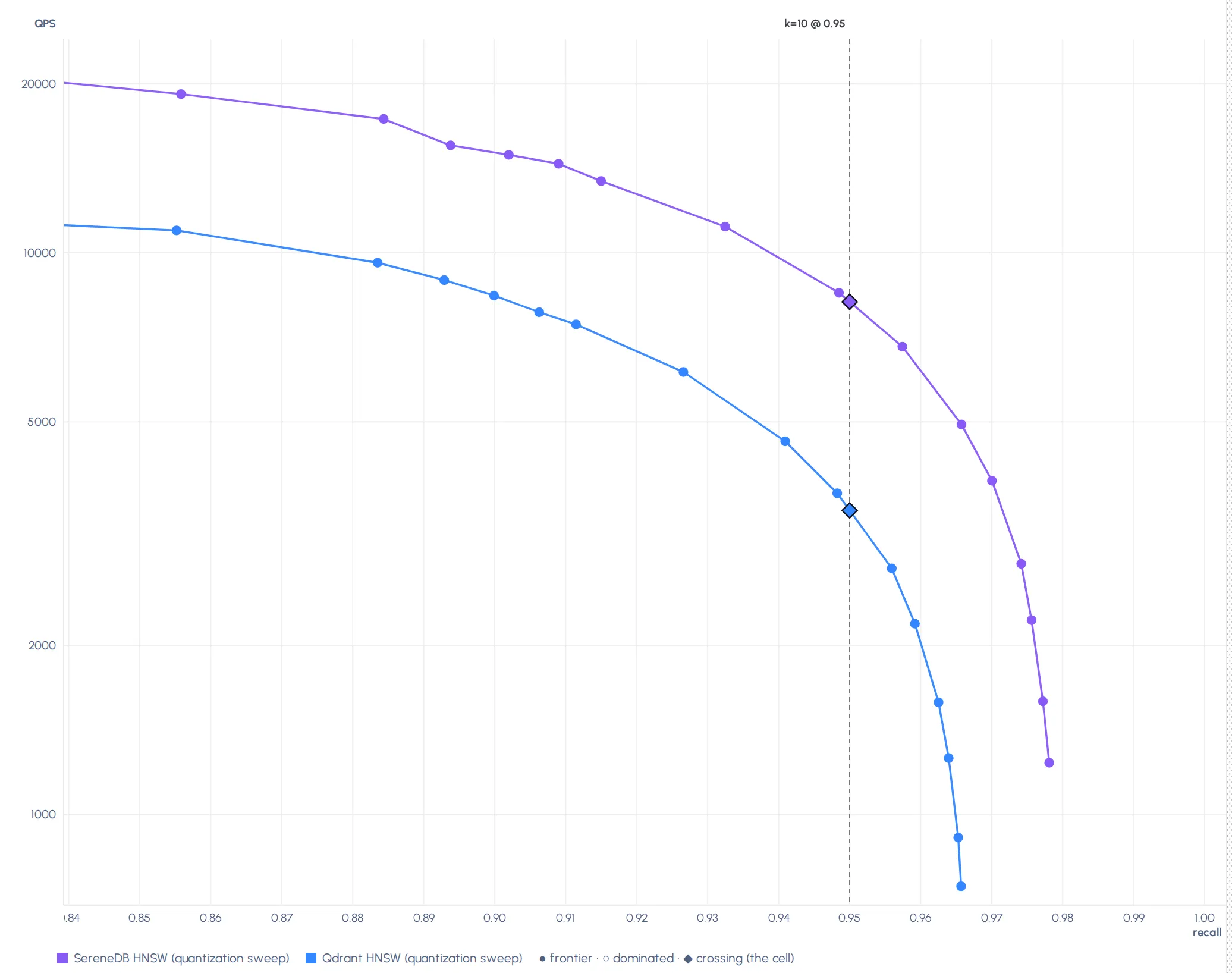
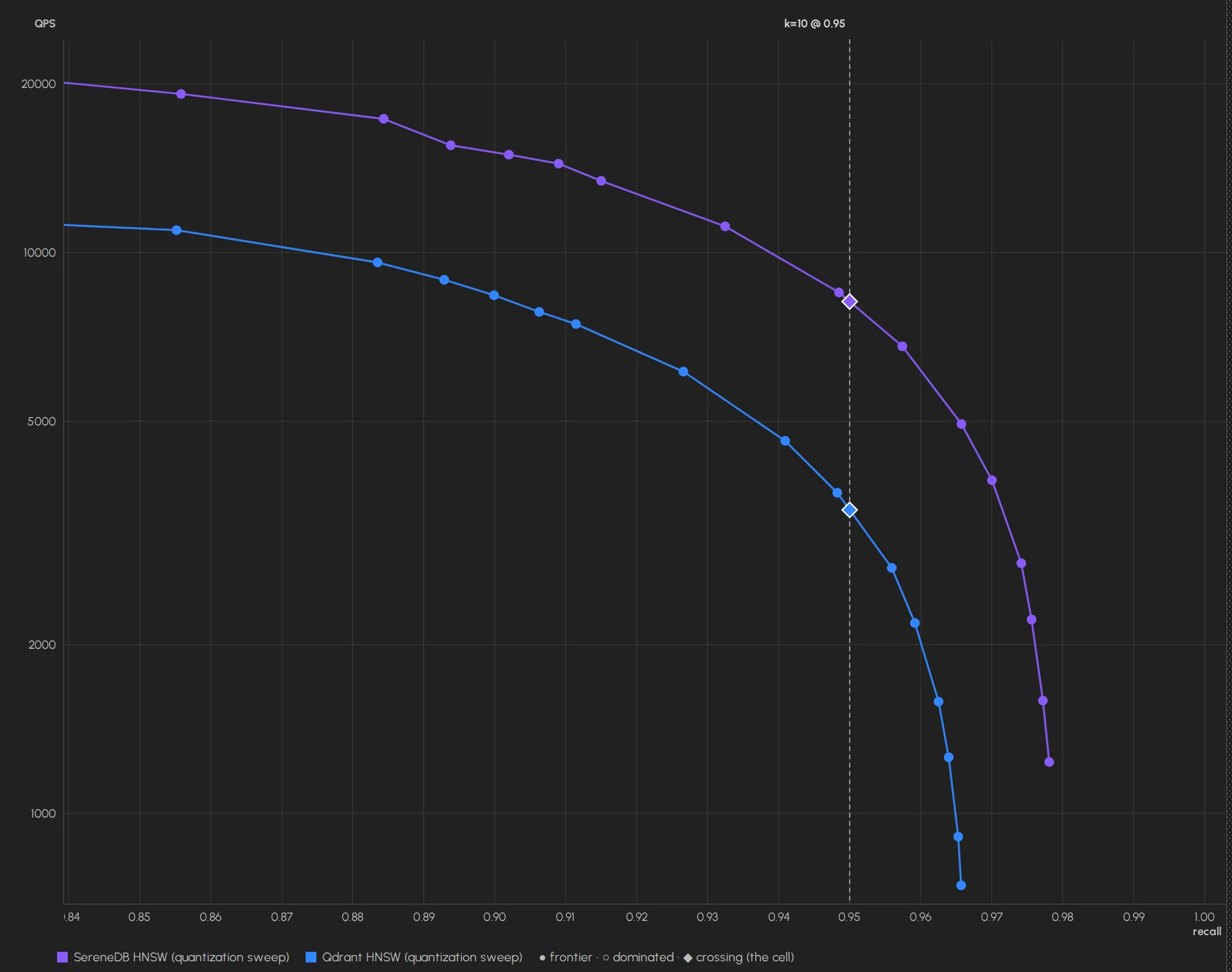
Unfiltered top-10: SereneDB's curve lies above Qdrant's everywhere, 15,079 against 8,381 queries per second at recall 0.90 and 8,177 against 3,477 at 0.95. It also reaches higher recall at the top (0.978 against 0.966).
SereneDB is faster in all 20 rows both engines reach: 1.8× to 2.4× unfiltered, 2.7× to 4.8× on the 10% filters, 6.6× on the query's own cluster at k = 1000 and 9.2× on another language. On the 1% filters and the far cluster Qdrant's recall stops at 0.90 to 0.93 at every beam, so those 11 rows are SereneDB's alone. Without reranking, 8-bit codes cap recall near 0.98 in both engines, so neither reaches the 0.99 rows. At 10M the 0.1% category and the far cluster keep fewer than ten times k rows at k = 1000, so those two rows are not asked.
Loading at this size is close: 776 s and 53 GB for SereneDB, 778 s and 56 GB for Qdrant. From a cold page cache SereneDB accepts queries after 3 s and answers its first vector query after 29 s, once it has read the graphs and codes. Qdrant answers nothing for 25 s, then everything.
Why the gap is smaller in RAM
Nothing is reread here, so the lead is what the walk, the distances on codes and the filters give: 1.8× to 2.4× unfiltered, about the same as the walk alone at 247M. At 247M the rereads multiply it, because Qdrant reads 2× to 5× more from disk per query and the difference grows with k.
At thousands of queries per second, the work around the index starts to count as well: parsing, planning and scheduling each query. SereneDB's executor is built for mixed workloads, where short queries run next to long analytical ones. It splits each query into small pieces of work that a shared pool of workers picks up, with accounting per session, so thousands of short queries share the cores with each other and with the long ones.
The filters make the biggest difference here too. Without per-value graphs, Qdrant's filtered walk stops below recall 0.95 on the 1% filters and the far cluster. SereneDB scores the matching rows directly in segments where a filter leaves few of them, so it reaches 0.95 there at 1,200 to 1,600 queries per second. On the far cluster it does 17,000 to 20,000.
Don't trust us, run VectorBench yourself
Everything is in the repository: the dataset preparation, both participants with their settings and ladders plus the result files this post is drawn from.
git clone https://github.com/serenedb/vectorbench
cd vectorbench
uv venv .venv && uv pip install --python .venv/bin/python -e .
export PYTHONPATH=lib VECTORBENCH_DATA_DIR=/path/to/data
.venv/bin/python -m vectorbench.cli prepare --dataset wiki-v3-1024-247m
.venv/bin/python -m vectorbench.cli run --participant serenedb-hnsw-quant --dataset wiki-v3-1024-247m --index \
    --views throughput --point-queries 10=1000,100=500,1000=200 --evict --warmup 0 --settle 0 --startup-samples 1
Both participants, with every setting and ladder, are in the serenedb/vectorbench repository. PRs to either are welcome.
What's next
VectorBench will keep growing in two directions. More systems: Elasticsearch, OpenSearch, Milvus, pgvector and others. More cases, starting with the tier this post leaves out: machines where even the graph and codes don't fit in RAM, which call for fully on-disk indexes such as IVF or DiskANN-style graphs. Each comes as its own participant directory with settings, ladders and results, the same way as these two.
One system
On 247 million vectors, with their terabyte of floats on disk and read only to rerank, SereneDB was faster than Qdrant in every approximate row both could answer, by 1.3× to 14×. It also answered five rows Qdrant could not. On ten million vectors in RAM it was faster in every row both could answer, by 1.5× to 9.2×. Eleven more rows only SereneDB answered.
The usual argument for a dedicated vector database next to the main one is speed. SereneDB does SQL, full-text search and analytics, and on vector search it beat a dedicated vector database at both sizes. In SereneDB the embedding is a column and the vector index is one column of the index that also serves text search and filters. A filtered nearest neighbour query is a WHERE and an ORDER BY in the same SQL statement as everything else. No second system to load, no payload to copy over and keep in sync.
docker run -d --name serenedb -p 7890:7890 serenedb/serenedb
That is the whole install. The quick start takes it from there. If your results look different, open an issue and show us.
If you find this interesting, we'd be grateful if you support SereneDB with a star on GitHub. For an early-stage project, it means more than you might think.
If you'd like to see more open benchmarks: