

Window Functions
SereneDB supports window functions, which can use multiple rows to calculate a value for each row. Window functions are blocking operators, i.e., they require their entire input to be buffered, making them one of the most memory-intensive operators in SQL.
Window functions are available in SQL since SQL:2003 and are supported by major SQL database systems.
Examples
Generate a row_number column to enumerate rows:
SELECT row_number() OVER () AS row_numberFROM salesORDER BY 1; row_number
------------
1
2
3
4Generate a row_number column to enumerate rows, ordered by time:
SELECT row_number() OVER (ORDER BY time)FROM sales; row_number
------------
1
2
3
4Generate a row_number column to enumerate rows, ordered by time and partitioned by region:
SELECT row_number() OVER (PARTITION BY region ORDER BY time)FROM sales; row_number
------------
1
1
2
2Compute the difference between the current and the previous-by-time amount:
SELECT amount - lag(amount) OVER (ORDER BY time)FROM sales; difference
------------
NULL
150
-70
40Compute the percentage of the total amount of sales per region for each row:
SELECT amount / sum(amount) OVER (PARTITION BY region) AS percentageFROM sales; percentage
------------
0.2857
0.7143
0.45
0.55Syntax
Window functions can only be used in the SELECT clause. To share OVER specifications between functions, use the statement's WINDOW clause and use the OVER ⟨window_name⟩ syntax.
General-Purpose Window Functions
The table below shows the available general window functions.
| Name | Description |
|---|---|
cume_dist([ORDER BY ordering]) | The cumulative distribution: (number of partition rows preceding or peer with current row) / total partition rows. |
dense_rank() | The rank of the current row without gaps; this function counts peer groups. |
fill(expr [ ORDER BY ordering]) | Fill in missing values using linear interpolation with ORDER BY as the X-axis. |
first_value(expr[ ORDER BY ordering][ IGNORE NULLS]) | Returns expr evaluated at the row that is the first row (with a non-null value of expr if IGNORE NULLS is set) of the window frame. |
lag(expr[, offset[, default]][ ORDER BY ordering][ IGNORE NULLS]) | Returns expr evaluated at the row that is offset rows (among rows with a non-null value of expr if IGNORE NULLS is set) before the current row within the window frame; if there is no such row, instead return default (which must be of the same type as expr). Both offset and default are evaluated with respect to the current row. If omitted, offset defaults to 1 and default to NULL. |
last_value(expr[ ORDER BY ordering][ IGNORE NULLS]) | Returns expr evaluated at the row that is the last row (among rows with a non-null value of expr if IGNORE NULLS is set) of the window frame. |
lead(expr[, offset[, default]][ ORDER BY ordering][ IGNORE NULLS]) | Returns expr evaluated at the row that is offset rows after the current row (among rows with a non-null value of expr if IGNORE NULLS is set) within the window frame; if there is no such row, instead return default (which must be of the same type as expr). Both offset and default are evaluated with respect to the current row. If omitted, offset defaults to 1 and default to NULL. |
nth_value(expr, nth[ ORDER BY ordering][ IGNORE NULLS]) | Returns expr evaluated at the nth row (among rows with a non-null value of expr if IGNORE NULLS is set) of the window frame (counting from 1); NULL if no such row. |
ntile(num_buckets[ ORDER BY ordering]) | An integer ranging from 1 to num_buckets, dividing the partition as equally as possible. |
percent_rank([ORDER BY ordering]) | The relative rank of the current row: (rank() - 1) / (total partition rows - 1). |
rank([ORDER BY ordering]) | The rank of the current row with gaps; same as row_number of its first peer. |
row_number([ORDER BY ordering]) | The number of the current row within the partition, counting from 1. |
cume_dist([ORDER BY ordering])
| Description | The cumulative distribution: (number of partition rows preceding or peer with current row) / total partition rows. If an ORDER BY clause is specified, the distribution is computed within the frame using the provided ordering instead of the frame ordering. |
|---|---|
| Return type | DOUBLE |
| Example | cume_dist() |
dense_rank()
| Description | The rank of the current row without gaps; this function counts peer groups. |
|---|---|
| Return type | BIGINT |
| Example | dense_rank() |
| Aliases | rank_dense() |
fill(expr[ ORDER BY ordering])
| Description | Replaces NULL values of expr with a linear interpolation based on the closest non-NULL values and the sort values. Both values must support arithmetic and there must be only one ordering key. For missing values at the ends, linear extrapolation is used. Failure to interpolate results in the NULL value being retained. |
|---|---|
| Return type | Same type as expr |
| Example | fill(column) |
first_value(expr[ ORDER BY ordering][ IGNORE NULLS])
| Description | Returns expr evaluated at the row that is the first row (with a non-null value of expr if IGNORE NULLS is set) of the window frame. If an ORDER BY clause is specified, the first row number is computed within the frame using the provided ordering instead of the frame ordering. |
|---|---|
| Return type | Same type as expr |
| Example | first_value(column) |
lag(expr[, offset[, default]][ ORDER BY ordering][ IGNORE NULLS])
| Description | Returns expr evaluated at the row that is offset rows (among rows with a non-null value of expr if IGNORE NULLS is set) before the current row within the window frame; if there is no such row, instead return default (which must be of the same type as expr). Both offset and default are evaluated with respect to the current row. If omitted, offset defaults to 1 and default to NULL. If an ORDER BY clause is specified, the lagged row number is computed within the frame using the provided ordering instead of the frame ordering. |
|---|---|
| Return type | Same type as expr |
| Example | lag(column, 3, 0) |
last_value(expr[ ORDER BY ordering][ IGNORE NULLS])
| Description | Returns expr evaluated at the row that is the last row (among rows with a non-null value of expr if IGNORE NULLS is set) of the window frame. If omitted, offset defaults to 1 and default to NULL. If an ORDER BY clause is specified, the last row is determined within the frame using the provided ordering instead of the frame ordering. |
|---|---|
| Return type | Same type as expr |
| Example | last_value(column) |
lead(expr[, offset[, default]][ ORDER BY ordering][ IGNORE NULLS])
| Description | Returns expr evaluated at the row that is offset rows after the current row (among rows with a non-null value of expr if IGNORE NULLS is set) within the window frame; if there is no such row, instead return default (which must be of the same type as expr). Both offset and default are evaluated with respect to the current row. If omitted, offset defaults to 1 and default to NULL. If an ORDER BY clause is specified, the leading row number is computed within the frame using the provided ordering instead of the frame ordering. |
|---|---|
| Return type | Same type as expr |
| Example | lead(column, 3, 0) |
nth_value(expr, nth[ ORDER BY ordering][ IGNORE NULLS])
| Description | Returns expr evaluated at the nth row (among rows with a non-null value of expr if IGNORE NULLS is set) of the window frame (counting from 1); NULL if no such row. If an ORDER BY clause is specified, the nth row number is computed within the frame using the provided ordering instead of the frame ordering. |
|---|---|
| Return type | Same type as expr |
| Example | nth_value(column, 2) |
ntile(num_buckets[ ORDER BY ordering])
| Description | An integer ranging from 1 to num_buckets, dividing the partition as equally as possible. If an ORDER BY clause is specified, the ntile is computed within the frame using the provided ordering instead of the frame ordering. |
|---|---|
| Return type | BIGINT |
| Example | ntile(4) |
percent_rank([ORDER BY ordering])
| Description | The relative rank of the current row: (rank() - 1) / (total partition rows - 1). If an ORDER BY clause is specified, the relative rank is computed within the frame using the provided ordering instead of the frame ordering. |
|---|---|
| Return type | DOUBLE |
| Example | percent_rank() |
rank([ORDER BY ordering])
| Description | The rank of the current row with gaps; same as row_number of its first peer. If an ORDER BY clause is specified, the rank is computed within the frame using the provided ordering instead of the frame ordering. |
|---|---|
| Return type | BIGINT |
| Example | rank() |
row_number([ORDER BY ordering])
| Description | The number of the current row within the partition, counting from 1. If an ORDER BY clause is specified, the row number is computed within the frame using the provided ordering instead of the frame ordering. |
|---|---|
| Return type | BIGINT |
| Example | row_number() |
Aggregate Window Functions
All aggregate functions can be used in a windowing context, including the optional FILTER clause.
The first and last aggregate functions are shadowed by the respective general-purpose window functions, with the minor consequence that the FILTER clause is not available for these but IGNORE NULLS is.
DISTINCT Arguments
All aggregate window functions support using a DISTINCT clause for the arguments. When the DISTINCT clause is
provided, only distinct values are considered in the computation of the aggregate. This is typically used in combination
with the COUNT aggregate to get the number of distinct elements; but it can be used together with any aggregate
function in the system. There are some aggregates that are insensitive to duplicate values (e.g., min, max) and for
them this clause is parsed and ignored.
-- Count the number of distinct names at a given point in timeSELECT count(DISTINCT name) OVER (ORDER BY time) FROM sales; count
-------
1
2
2
3ORDER BY Arguments
All aggregate window functions support using an ORDER BY argument clause that is different from the window ordering.
When the ORDER BY argument clause is provided, the values being aggregated are sorted before applying the function.
Usually this is not important, but there are some order-sensitive aggregates that can have indeterminate results (e.g.,
mode, list and string_agg). These can be made deterministic by ordering the arguments. For order-insensitive
aggregates, this clause is parsed and ignored.
-- Compute the modal value up to each time, breaking ties in favor of the most recent valueSELECT mode(value ORDER BY time DESC) OVER (ORDER BY time) FROM sales;mode ------ 42 84 42 42
The SQL standard does not provide for using ORDER BY with general-purpose window functions, but we have extended all
of these functions (except dense_rank) to accept this syntax and use framing to restrict the range that the secondary
ordering applies to.
SELECT event, athlete, first_value(athlete ORDER BY time) OVER w AS fastestFROM resultsWINDOW w AS (PARTITION BY event ORDER BY date)ORDER BY event, athlete;event | athlete | fastest -------+---------+--------- 100m | Ada | Ada 100m | Bob | Bob 200m | Cy | Cy
Note that there is no comma separating the arguments from the ORDER BY clause.
Nulls
All general-purpose window functions that accept IGNORE NULLS respect nulls by default. This default behavior can optionally be made explicit via RESPECT NULLS.
In contrast, all aggregate window functions (except for list and its aliases, which can be made to ignore nulls via a FILTER) ignore nulls and do not accept RESPECT NULLS. For example, sum(column) OVER (ORDER BY time) AS cumulativeColumn computes a cumulative sum where rows with a NULL value of column have the same value of cumulativeColumn as the row that precedes them.
Evaluation
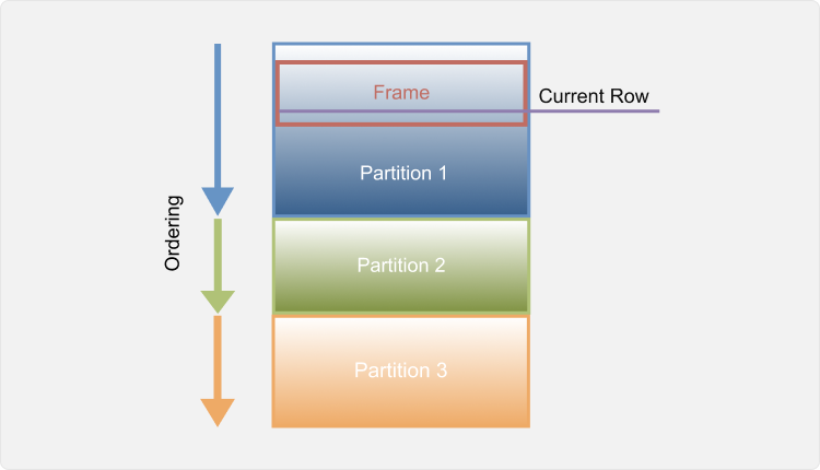
Windowing works by breaking a relation up into independent partitions, ordering those partitions, and then computing a new column for each row as a function of the nearby values. Some window functions depend only on the partition boundary and the ordering, but a few (including all the aggregates) also use a frame. Frames are specified as a number of rows on either side (preceding or following) of the current row. The distance can be specified as a number of rows, as a range of values using the partition's ordering value and a distance, or as a number of groups (sets of rows with the same sort value).
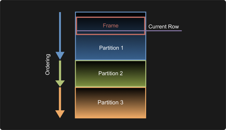
The full syntax is shown in the diagram at the top of the page, and this diagram visually illustrates computation environment:
Partition and Ordering
Partitioning breaks the relation up into independent, unrelated pieces. Partitioning is optional, and if none is specified then the entire relation is treated as a single partition. Window functions cannot access values outside of the partition containing the row they are being evaluated at.
Ordering is also optional, but without it the results of general-purpose window functions and order-sensitive aggregate functions, and the order of framing are not well-defined. Each partition is ordered using the same ordering clause.
Here is a table of power generation data. To load it from a CSV file, run:
CREATE TABLE "Generation History" AS FROM 'power-plant-generation-history.csv';After partitioning by plant and ordering by date, it will have this layout:
SELECT "Plant", "Date", "MWh"FROM "Generation History"ORDER BY "Plant", "Date";Plant | Date | MWh -----------+------------+-------- Boston | 2019-01-02 | 564337 Boston | 2019-01-03 | 507405 Boston | 2019-01-04 | 528523 Boston | 2019-01-05 | 469538 Boston | 2019-01-06 | 474163 Boston | 2019-01-07 | 507213 Boston | 2019-01-08 | 613040 Boston | 2019-01-09 | 582588 Boston | 2019-01-10 | 499506 Boston | 2019-01-11 | 482014 Boston | 2019-01-12 | 486134 Boston | 2019-01-13 | 531518 Worcester | 2019-01-02 | 118860 Worcester | 2019-01-03 | 101977 Worcester | 2019-01-04 | 106054 Worcester | 2019-01-05 | 92182 Worcester | 2019-01-06 | 94492 Worcester | 2019-01-07 | 99932 Worcester | 2019-01-08 | 118854 Worcester | 2019-01-09 | 113506 Worcester | 2019-01-10 | 96644 Worcester | 2019-01-11 | 93806 Worcester | 2019-01-12 | 98963 Worcester | 2019-01-13 | 107170
In what follows, we shall use this table (or small sections of it) to illustrate various pieces of window function evaluation.
The simplest window function is row_number().
This function just computes the 1-based row number within the partition using the query:
SELECT "Plant", "Date", row_number() OVER (PARTITION BY "Plant" ORDER BY "Date") AS "Row"FROM "Generation History";Plant | Date | Row -----------+------------+----- Boston | 2019-01-02 | 1 Boston | 2019-01-03 | 2 Boston | 2019-01-04 | 3 Boston | 2019-01-05 | 4 Boston | 2019-01-06 | 5 Boston | 2019-01-07 | 6 Boston | 2019-01-08 | 7 Boston | 2019-01-09 | 8 Boston | 2019-01-10 | 9 Boston | 2019-01-11 | 10 Boston | 2019-01-12 | 11 Boston | 2019-01-13 | 12 Worcester | 2019-01-02 | 1 Worcester | 2019-01-03 | 2 Worcester | 2019-01-04 | 3 Worcester | 2019-01-05 | 4 Worcester | 2019-01-06 | 5 Worcester | 2019-01-07 | 6 Worcester | 2019-01-08 | 7 Worcester | 2019-01-09 | 8 Worcester | 2019-01-10 | 9 Worcester | 2019-01-11 | 10 Worcester | 2019-01-12 | 11 Worcester | 2019-01-13 | 12
The row number restarts at 1 for each Plant partition.
Note that even though the function is computed with an ORDER BY clause,
the result does not have to be sorted,
so the SELECT also needs to be explicitly sorted if that is desired.
Framing
Framing specifies a set of rows relative to each row where the function is evaluated.
The distance from the current row is given as an expression either PRECEDING or FOLLOWING the current row in the order specified by the ORDER BY clause in the OVER specification.
This distance can either be specified as an integral number of ROWS or GROUPS,
or as a RANGE delta expression. It is invalid for a frame to start after it ends.
For a RANGE specification, there must be only one ordering expression and it must support subtraction unless only the sentinel boundary values UNBOUNDED PRECEDING / UNBOUNDED FOLLOWING / CURRENT ROW are used.
Using the EXCLUDE clause, rows comparing equal to the current row in the specified ordering expression (so-called peers) can be excluded from the frame.
The default frame is unbounded (i.e., the entire partition) when no ORDER BY clause is present and RANGE BETWEEN UNBOUNDED PRECEDING AND CURRENT ROW when an ORDER BY clause is present. By default, the CURRENT ROW boundary value (but not the CURRENT ROW in the EXCLUDE clause) means the current row and all its peers when RANGE or GROUP framing are used but it means only the current row when ROWS framing is used.
ROWS Framing
Here is a simple ROW frame query, using an aggregate function:
SELECT points, sum(points) OVER ( ORDER BY datetime ROWS BETWEEN 1 PRECEDING AND 1 FOLLOWING) AS "Moving Sum"FROM resultsORDER BY datetime; points | Moving Sum
--------+------------
10 | 19
9 | 31
12 | 21This query computes the sum of each point and the points on either side of it:
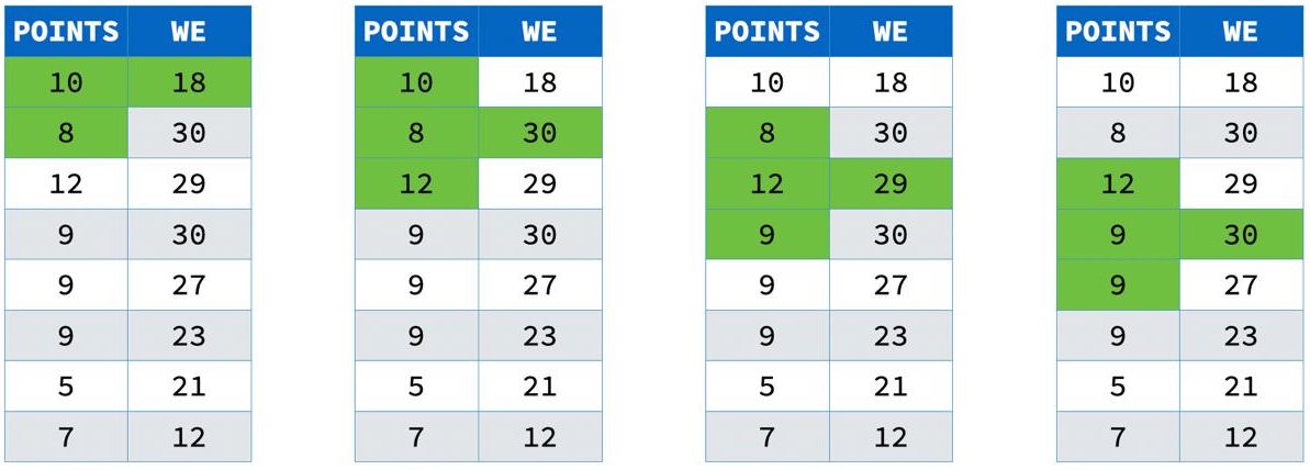
Notice that at the edge of the partition, there are only two values added together. This is because frames are cropped to the edge of the partition.
RANGE Framing
Returning to the power data, suppose the data is noisy. We might want to compute a 7 day moving average for each plant to smooth out the noise. To do this, we can use this window query:
SELECT "Plant", "Date", avg("MWh") OVER ( PARTITION BY "Plant" ORDER BY "Date" ASC RANGE BETWEEN INTERVAL 3 DAYS PRECEDING AND INTERVAL 3 DAYS FOLLOWING) AS "MWh 7-day Moving Average"FROM "Generation History";Plant | Date | MWh 7-day Moving Average -----------+------------+-------------------------- Boston | 2019-01-02 | 517450.75 Boston | 2019-01-03 | 508793.2 Boston | 2019-01-04 | 508529.8333333333 Boston | 2019-01-05 | 523459.85714285716 Boston | 2019-01-06 | 526067.1428571428 Boston | 2019-01-07 | 524938.7142857143 Boston | 2019-01-08 | 518294.5714285714 Boston | 2019-01-09 | 520665.4285714286 Boston | 2019-01-10 | 528859 Boston | 2019-01-11 | 532466.6666666666 Boston | 2019-01-12 | 516352 Boston | 2019-01-13 | 499793 Worcester | 2019-01-02 | 104768.25 Worcester | 2019-01-03 | 102713 Worcester | 2019-01-04 | 102249.5 Worcester | 2019-01-05 | 104621.57142857143 Worcester | 2019-01-06 | 103856.71428571429 Worcester | 2019-01-07 | 103094.85714285714 Worcester | 2019-01-08 | 101345.14285714286 Worcester | 2019-01-09 | 102313.85714285714 Worcester | 2019-01-10 | 104125 Worcester | 2019-01-11 | 104823.83333333333 Worcester | 2019-01-12 | 102017.8 Worcester | 2019-01-13 | 99145.75
This query partitions the data by Plant (to keep the different power plants' data separate),
orders each plant's partition by Date (to put the energy measurements next to each other),
and uses a RANGE frame of three days on either side of each day for the avg
(to handle any missing days).
GROUPS Framing
The third type of framing counts groups of rows relative the current row.
A group in this framing is a set of values with identical ORDER BY values.
If we assume that power is being generated on every day,
we can use GROUPS framing to compute the moving average of all power generated in the system
without having to resort to date arithmetic:
SELECT "Date", "Plant", avg("MWh") OVER ( ORDER BY "Date" ASC GROUPS BETWEEN 3 PRECEDING AND 3 FOLLOWING) AS "MWh 7-day Moving Average"FROM "Generation History";Date | Plant | MWh 7-day Moving Average ------------+-----------+-------------------------- 2019-01-02 | Boston | 311109.5 2019-01-02 | Worcester | 311109.5 2019-01-03 | Boston | 305753.1 2019-01-03 | Worcester | 305753.1 2019-01-04 | Boston | 305389.6666666667 2019-01-04 | Worcester | 305389.6666666667 2019-01-05 | Boston | 314040.71428571426 2019-01-05 | Worcester | 314040.71428571426 2019-01-06 | Boston | 314961.9285714286 2019-01-06 | Worcester | 314961.9285714286 2019-01-07 | Boston | 314016.78571428574 2019-01-07 | Worcester | 314016.78571428574 2019-01-08 | Boston | 309819.85714285716 2019-01-08 | Worcester | 309819.85714285716 2019-01-09 | Boston | 311489.64285714284 2019-01-09 | Worcester | 311489.64285714284 2019-01-10 | Boston | 316492 2019-01-10 | Worcester | 316492 2019-01-11 | Boston | 318645.25 2019-01-11 | Worcester | 318645.25 2019-01-12 | Boston | 309184.9 2019-01-12 | Worcester | 309184.9 2019-01-13 | Boston | 299469.375 2019-01-13 | Worcester | 299469.375
Notice how the values for each date are the same.
EXCLUDE Clause
EXCLUDE is an optional modifier to the frame clause for excluding rows around the CURRENT ROW.
This is useful when you want to compute some aggregate value of nearby rows
to see how the current row compares to it.
In the following example, we want to know how an athlete's time in an event compares to the average of all the times recorded for their event within ±10 days:
SELECT event, date, athlete, avg(time) OVER w AS recentFROM resultsWINDOW w AS ( PARTITION BY event ORDER BY date RANGE BETWEEN INTERVAL 10 DAYS PRECEDING AND INTERVAL 10 DAYS FOLLOWING EXCLUDE CURRENT ROW);event | date | athlete | recent -------+------------+---------+-------- 100m | 2025-01-01 | Ada | 12.1 100m | 2025-01-02 | Bob | 12.3 200m | 2025-01-01 | Cy | NULL
There are four options for EXCLUDE that specify how to treat the current row:
CURRENT ROW– exclude just the current rowGROUP– exclude the current row and all its “peers” (rows that have the sameORDER BYvalue)TIES– exclude all peer rows, but not the current row (this makes a hole on either side)NO OTHERS– don't exclude anything (the default)
Exclusion is implemented for both windowed aggregates as well as for the first, last and nth_value functions.
WINDOW Clauses
Multiple different OVER clauses can be specified in the same SELECT, and each will be computed separately.
Often, however, we want to use the same layout for multiple window functions.
The WINDOW clause can be used to define a named window that can be shared between multiple window functions:
SELECT "Plant", "Date", min("MWh") OVER seven AS "MWh 7-day Moving Minimum", avg("MWh") OVER seven AS "MWh 7-day Moving Average", max("MWh") OVER seven AS "MWh 7-day Moving Maximum"FROM "Generation History"WINDOW seven AS ( PARTITION BY "Plant" ORDER BY "Date" ASC RANGE BETWEEN INTERVAL 3 DAYS PRECEDING AND INTERVAL 3 DAYS FOLLOWING);Plant | Date | MWh 7-day Moving Minimum | MWh 7-day Moving Average | MWh 7-day Moving Maximum -----------+------------+--------------------------+--------------------------+-------------------------- Boston | 2019-01-02 | 469538 | 517450.75 | 564337 Boston | 2019-01-03 | 469538 | 508793.2 | 564337 Boston | 2019-01-04 | 469538 | 508529.8333333333 | 564337 Boston | 2019-01-05 | 469538 | 523459.85714285716 | 613040 Boston | 2019-01-06 | 469538 | 526067.1428571428 | 613040 Boston | 2019-01-07 | 469538 | 524938.7142857143 | 613040 Boston | 2019-01-08 | 469538 | 518294.5714285714 | 613040 Boston | 2019-01-09 | 474163 | 520665.4285714286 | 613040 Boston | 2019-01-10 | 482014 | 528859 | 613040 Boston | 2019-01-11 | 482014 | 532466.6666666666 | 613040 Boston | 2019-01-12 | 482014 | 516352 | 582588 Boston | 2019-01-13 | 482014 | 499793 | 531518 Worcester | 2019-01-02 | 92182 | 104768.25 | 118860 Worcester | 2019-01-03 | 92182 | 102713 | 118860 Worcester | 2019-01-04 | 92182 | 102249.5 | 118860 Worcester | 2019-01-05 | 92182 | 104621.57142857143 | 118860 Worcester | 2019-01-06 | 92182 | 103856.71428571429 | 118854 Worcester | 2019-01-07 | 92182 | 103094.85714285714 | 118854 Worcester | 2019-01-08 | 92182 | 101345.14285714286 | 118854 Worcester | 2019-01-09 | 93806 | 102313.85714285714 | 118854 Worcester | 2019-01-10 | 93806 | 104125 | 118854 Worcester | 2019-01-11 | 93806 | 104823.83333333333 | 118854 Worcester | 2019-01-12 | 93806 | 102017.8 | 113506 Worcester | 2019-01-13 | 93806 | 99145.75 | 107170
The three window functions will also share the data layout, which will improve performance.
Multiple windows can be defined in the same WINDOW clause by comma-separating them:
SELECT "Plant", "Date", min("MWh") OVER seven AS "MWh 7-day Moving Minimum", avg("MWh") OVER seven AS "MWh 7-day Moving Average", max("MWh") OVER seven AS "MWh 7-day Moving Maximum", min("MWh") OVER three AS "MWh 3-day Moving Minimum", avg("MWh") OVER three AS "MWh 3-day Moving Average", max("MWh") OVER three AS "MWh 3-day Moving Maximum"FROM "Generation History"WINDOW seven AS ( PARTITION BY "Plant" ORDER BY "Date" ASC RANGE BETWEEN INTERVAL 3 DAYS PRECEDING AND INTERVAL 3 DAYS FOLLOWING), three AS ( PARTITION BY "Plant" ORDER BY "Date" ASC RANGE BETWEEN INTERVAL 1 DAYS PRECEDING AND INTERVAL 1 DAYS FOLLOWING);Plant | Date | MWh 7-day Moving Minimum | MWh 7-day Moving Average | MWh 7-day Moving Maximum | MWh 3-day Moving Minimum | MWh 3-day Moving Average | MWh 3-day Moving Maximum -----------+------------+--------------------------+--------------------------+--------------------------+--------------------------+--------------------------+-------------------------- Boston | 2019-01-02 | 469538 | 517450.75 | 564337 | 507405 | 535871 | 564337 Boston | 2019-01-03 | 469538 | 508793.2 | 564337 | 507405 | 533421.6666666666 | 564337 Boston | 2019-01-04 | 469538 | 508529.8333333333 | 564337 | 469538 | 501822 | 528523 Boston | 2019-01-05 | 469538 | 523459.85714285716 | 613040 | 469538 | 490741.3333333333 | 528523 Boston | 2019-01-06 | 469538 | 526067.1428571428 | 613040 | 469538 | 483638 | 507213 Boston | 2019-01-07 | 469538 | 524938.7142857143 | 613040 | 474163 | 531472 | 613040 Boston | 2019-01-08 | 469538 | 518294.5714285714 | 613040 | 507213 | 567613.6666666666 | 613040 Boston | 2019-01-09 | 474163 | 520665.4285714286 | 613040 | 499506 | 565044.6666666666 | 613040 Boston | 2019-01-10 | 482014 | 528859 | 613040 | 482014 | 521369.3333333333 | 582588 Boston | 2019-01-11 | 482014 | 532466.6666666666 | 613040 | 482014 | 489218 | 499506 Boston | 2019-01-12 | 482014 | 516352 | 582588 | 482014 | 499888.6666666667 | 531518 Boston | 2019-01-13 | 482014 | 499793 | 531518 | 486134 | 508826 | 531518 Worcester | 2019-01-02 | 92182 | 104768.25 | 118860 | 101977 | 110418.5 | 118860 Worcester | 2019-01-03 | 92182 | 102713 | 118860 | 101977 | 108963.66666666667 | 118860 Worcester | 2019-01-04 | 92182 | 102249.5 | 118860 | 92182 | 100071 | 106054 Worcester | 2019-01-05 | 92182 | 104621.57142857143 | 118860 | 92182 | 97576 | 106054 Worcester | 2019-01-06 | 92182 | 103856.71428571429 | 118854 | 92182 | 95535.33333333333 | 99932 Worcester | 2019-01-07 | 92182 | 103094.85714285714 | 118854 | 94492 | 104426 | 118854 Worcester | 2019-01-08 | 92182 | 101345.14285714286 | 118854 | 99932 | 110764 | 118854 Worcester | 2019-01-09 | 93806 | 102313.85714285714 | 118854 | 96644 | 109668 | 118854 Worcester | 2019-01-10 | 93806 | 104125 | 118854 | 93806 | 101318.66666666667 | 113506 Worcester | 2019-01-11 | 93806 | 104823.83333333333 | 118854 | 93806 | 96471 | 98963 Worcester | 2019-01-12 | 93806 | 102017.8 | 113506 | 93806 | 99979.66666666667 | 107170 Worcester | 2019-01-13 | 93806 | 99145.75 | 107170 | 98963 | 103066.5 | 107170
The queries above do not use a number of clauses commonly found in select statements, like
WHERE, GROUP BY, etc. For more complex queries you can find where WINDOW clauses fall in
the canonical order of the SELECT statement.
Filtering the Results of Window Functions Using QUALIFY
Window functions are executed after the WHERE and HAVING clauses have been already evaluated, so it's not possible to use these clauses to filter the results of window functions
The QUALIFY clause avoids the need for a subquery or WITH clause to perform this filtering.
Box and Whisker Queries
All aggregates can be used as windowing functions, including the complex statistical functions. These function implementations have been optimized for windowing, and we can use the window syntax to write queries that generate the data for moving box-and-whisker plots:
SELECT "Plant", "Date", min("MWh") OVER seven AS "MWh 7-day Moving Minimum", quantile_cont("MWh", [0.25, 0.5, 0.75]) OVER seven AS "MWh 7-day Moving IQR", max("MWh") OVER seven AS "MWh 7-day Moving Maximum"FROM "Generation History"WINDOW seven AS ( PARTITION BY "Plant" ORDER BY "Date" ASC RANGE BETWEEN INTERVAL 3 DAYS PRECEDING AND INTERVAL 3 DAYS FOLLOWING); Plant | Date | MWh 7-day Moving Minimum | MWh 7-day Moving IQR | MWh 7-day Moving Maximum
-----------+------------+--------------------------+------------------------------+--------------------------
Boston | 2019-01-02 | 469538 | {497938.25,517964,537476.5} | 564337
Boston | 2019-01-03 | 469538 | {474163,507405,528523} | 564337
Boston | 2019-01-04 | 469538 | {482425.5,507309,523243.5} | 564337
Boston | 2019-01-05 | 469538 | {490688,507405,546430} | 613040
Boston | 2019-01-06 | 469538 | {490688,507405,555555.5} | 613040
Boston | 2019-01-07 | 469538 | {486834.5,507213,555555.5} | 613040
Boston | 2019-01-08 | 469538 | {478088.5,499506,544900.5} | 613040
Boston | 2019-01-09 | 474163 | {484074,499506,544900.5} | 613040
Boston | 2019-01-10 | 482014 | {492820,507213,557053} | 613040
Boston | 2019-01-11 | 482014 | {489477,515512,569820.5} | 613040
Boston | 2019-01-12 | 482014 | {486134,499506,531518} | 582588
Boston | 2019-01-13 | 482014 | {485104,492820,507509} | 531518
Worcester | 2019-01-02 | 92182 | {99528.25,104015.5,109255.5} | 118860
Worcester | 2019-01-03 | 92182 | {94492,101977,106054} | 118860
Worcester | 2019-01-04 | 92182 | {95852,100954.5,105034.75} | 118860
Worcester | 2019-01-05 | 92182 | {97212,101977,112454} | 118860
Worcester | 2019-01-06 | 92182 | {97212,101977,109780} | 118854
Worcester | 2019-01-07 | 92182 | {95568,99932,109780} | 118854
Worcester | 2019-01-08 | 92182 | {94149,96644,106719} | 118854
Worcester | 2019-01-09 | 93806 | {95568,98963,106719} | 118854
Worcester | 2019-01-10 | 93806 | {97803.5,99932,110338} | 118854
Worcester | 2019-01-11 | 93806 | {97223.75,103066.5,111922} | 118854
Worcester | 2019-01-12 | 93806 | {96644,98963,107170} | 113506
Worcester | 2019-01-13 | 93806 | {95934.5,97803.5,101014.75} | 107170